User Input

Suppose we perform a simple test using a YAML spec and the Python API. This should take less than 1 minute for the example below.

Example example_project/specs/experiment.yaml:

dataset: ds0
forecast_horizon: fh1  # fh1 = 30 minutes ahead, fh9 = 2 days ahead
model: m6
hyperparameter: hp1

Run the experiment in Python. On macOS, start Python with python3 if python is not available.

import pynnlf

pynnlf.run_experiment("example_project/specs/experiment.yaml")

To skip plot generation and save storage:

import pynnlf

pynnlf.run_experiment(
    "example_project/specs/experiment.yaml",
    plot_enabled=False,
)

Output

The tool generates the following outputs.

Name	Type	Description
E00001_cv_test/	Folder	Time series of observation, forecast, and residual for each cross-validation split
E00001_cv_train/	Folder	Time series of observation, forecast, and residual for each cross-validation split
E00001_cv1_plots/	Folder	Optional folder with plots for the first cross-validation fold when plot generation is enabled
E00001_models/	Folder	Saved models used or generated during the experiment
E00001_a1_experiment_result.csv	File	Accuracy (cross-validated test n-RMSE), stability, training time, and run seed
E00001_a2_hyperparameter.csv	File	Effective hyperparameters used for each model
E00001_a3_cross_validation_result.csv	File	Detailed results for each cross-validation split

The file a1_experiment_result.csv summarises the results, including the cross validated nRMSE, its standard deviation, run_seed, and seed_keys_overridden.

To aggregate multiple experiments into one recap, run recap_experiments to write a workspace-level a1_experiment_result.csv that includes the experiment_folder column.

experiment_no	exp_date	dataset_no	dataset	dataset_freq_min	dataset_length_week	forecast_horizon_min	train_pct	test_pct	model_no	hyperparameter_no	model_name	hyperparameter	run_seed	seed_keys_overridden	runtime_ms	train_RMSE	train_RMSE_stddev	test_RMSE	test_RMSE_stddev	train_nRMSE	train_nRMSE_stddev	test_nRMSE	test_nRMSE_stddev
E00001	15/09/2025	ds0	test	30	10	30	0.9	0.1	m6	hp1	m6_lr_hp1	num_features: 50	99		201.769185	17.33	0.206421	17.7066	1.82726	2.98206	0.03552	3.04686	0.31443

The file a3_cross_validation_result.csv provides the detailed cross-validation (CV) results, from CV1 to CV10.

Experiment Metrics

#	runtime_ms	train_MBE	train_MAE	train_RMSE	train_MAPE	train_MASE	train_fskill	train_R2	test_MBE	test_MAE	test_RMSE	test_MAPE	test_MASE	test_fskill	test_R2	train_nRMSE	test_nRMSE
1	193.2564	0	12.208	17.122	27.366	0.422	55.471	0.988	-0.1804	13.278	19.679	22.808	0.459	43.531	0.981	2.9463	3.3863
2	224.8719	0	12.337	17.495	27.347	0.423	54.817	0.988	-0.1443	12.332	16.346	18.905	0.423	49.006	0.987	3.0105	2.8127
3	251.0867	0	12.361	17.477	22.314	0.433	54.031	0.987	0.3318	11.965	16.321	60.409	0.419	58.022	0.989	3.0074	2.8084
4	174.1974	0	12.401	17.573	28.635	0.434	53.775	0.987	-0.8563	11.654	15.427	13.623	0.408	60.346	0.992	3.0239	2.6546
5	232.7249	0	12.281	17.020	22.091	0.435	54.565	0.988	1.2783	12.536	20.375	70.615	0.444	53.147	0.986	2.9287	3.5060
6	173.2767	0	12.322	17.467	28.530	0.436	53.491	0.987	-0.6225	12.436	16.567	12.690	0.440	61.224	0.991	3.0056	2.8508
7	233.0346	0	12.171	17.004	26.500	0.427	55.250	0.988	0.8754	13.685	20.516	27.756	0.480	47.485	0.981	2.9260	3.5303
8	212.3849	0	12.286	17.390	26.759	0.428	54.516	0.988	-0.7814	12.809	17.191	23.091	0.447	53.467	0.985	2.9924	2.9581
9	157.8457	0	12.330	17.417	28.242	0.435	53.965	0.988	-1.0170	12.308	16.923	10.919	0.434	58.189	0.989	2.9970	2.9120
10	165.0126	0	12.269	17.335	28.311	0.421	55.265	0.988	1.0148	12.840	17.721	11.193	0.441	44.110	0.979	2.9829	3.0493
mean	201.7692	0	12.2966	17.330	26.6095	0.4294	54.5146	0.9877	-0.0102	12.5843	17.7066	27.2009	0.4395	52.8527	0.986	2.9821	3.0469
stddev	33.2319	0	0.0693	0.2064	2.4352	0.00591	0.6866	0.00048	0.8405	0.5983	1.8273	21.106	0.02059	6.5729	0.00447	0.03552	0.31443

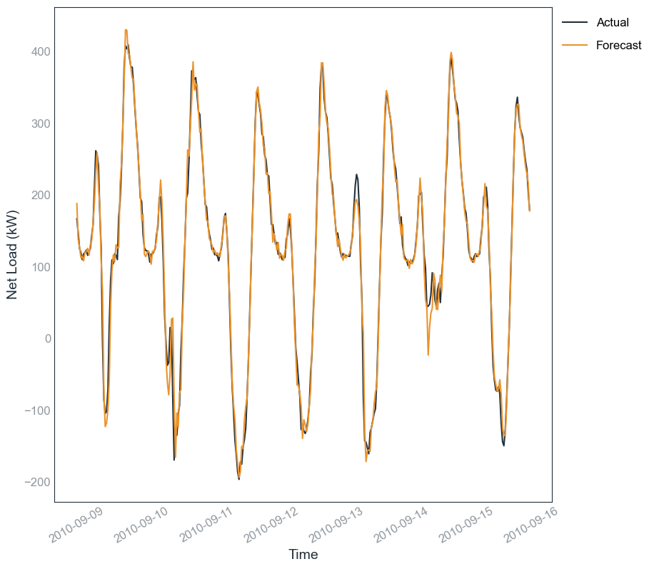
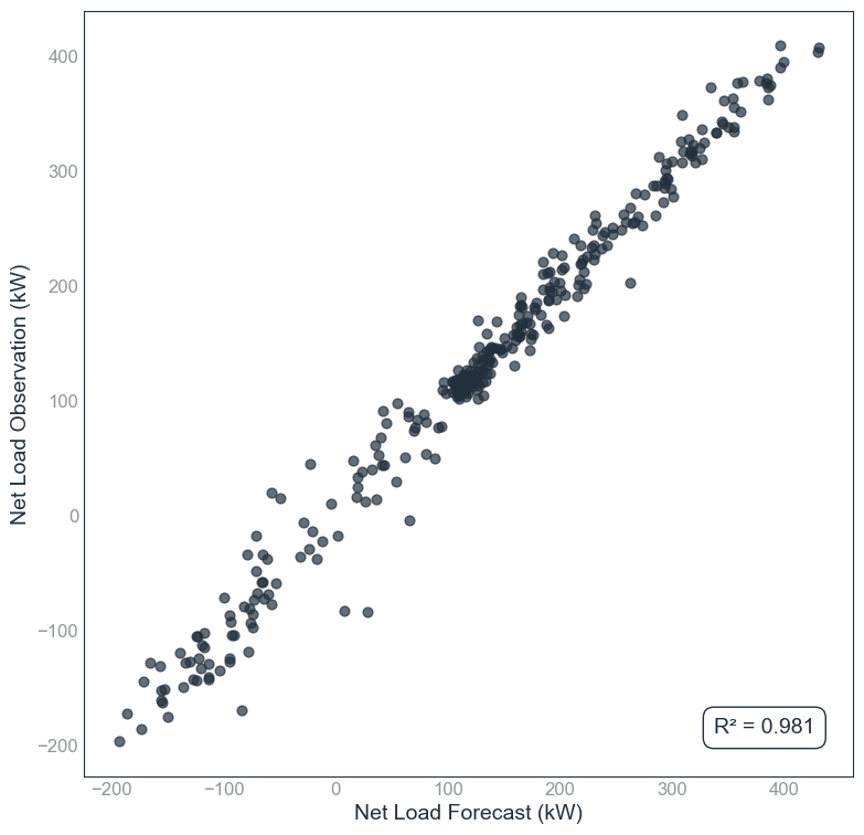
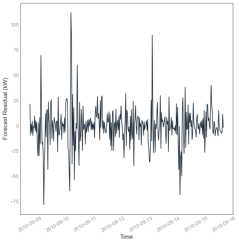
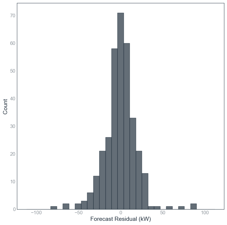
Below are some plots on the test set. These images are written only when plot generation is enabled:

Figure 1: Observation vs Forecast (Time Plot)	Figure 2: Observation vs Forecast (Scatter Plot)

Figure 3: Residuals Over Time	Figure 4: Residual Histogram